
Building a Real-Time Nigerian Stock Market Data Pipeline.
Building a Real-Time Nigerian Stock Market Analytics Pipeline: A data engineering and analytics project.


Introduction
The Nigerian Exchange (NGX) processes millions of naira in trades daily across various sectors, from banking giants such as GTCO Holdings to industrial powerhouses like Dangote Cement. But getting actionable insights from this market data requires more than just watching ticker symbols scroll by. It demands a robust data pipeline that can extract, transform, and visualize market movements to reveal opportunities.
In this post, I’ll walk you through how I built an end-to-end analytics platform for NGX equities data using Apache Airflow, PostgreSQL, and Tableau, one of the most used modern BI tools. Whether you’re a data engineer looking to build similar pipelines or an investor seeking to better understand market analytics, this project showcases practical patterns for real-time financial data processing.
The Challenge: Making Sense of Market Data
The Nigerian stock market data is publicly available through the NGX API, but raw data alone doesn’t answer the questions traders and analysts need:
Which stocks are gapping up or down at market open? (Price gaps often signal significant news or momentum)
How are different sectors performing? (Banking vs. Industrial Goods vs. Consumer Goods)
Who are the volume leaders? (High volume often precedes major price moves)
What’s the overall market breadth? (Are more stocks advancing or declining?)
To answer these questions at scale, I needed a system that could:
Fetch fresh data daily from the NGX API.
Store it reliably in a database.
Pre-compute complex analytics.
Serve insights through interactive dashboards.
Overview of Architecture
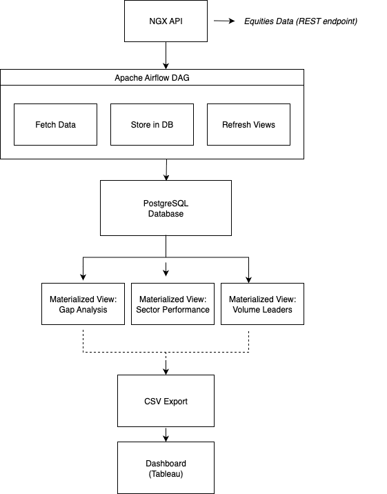
Implementation Deep Dive
Data Extraction with Apache Airflow
The pipeline starts with an Airflow DAG that runs daily at 3 PM WAT—30 minutes after the Nigerian market closes at 2:30 PM. This timing ensures we capture all the data from the trading day.
import requests
import pandas as pd
def fetch_ngx_equities(**kwargs):
base_url = “https://doclib.ngxgroup.com/REST/api/statistics/equities/”
all_data = []
page = 0
page_size = 300
while True:
url = f”{base_url}?market=§or=&orderby=&pageSize={page_size}&pageNo={page}”
print(f”Fetching page {page}”)
response = requests.get(url, timeout=15)
response.raise_for_status()
data = response.json()
# Handle if the response is a list or a dict
if isinstance(data, list):
items = data
elif isinstance(data, dict):
items = data.get(”data”, [])
else:
print(f”Unexpected data type: {type(data)}”)
break
if not items:
print(”No more data — done”)
break
all_data.extend(items)
page += 1
df = pd.DataFrame(all_data)
The function fetch_ngx_equities.py uses Python’s requests library to download the NGX daily equities data from the API endpoint. The function returns a DataFrame with all the raw equity records. The API returns paginated data with 300 records per page, so we loop through all pages to capture the full market (typically 150-200 listed equities). Key data points include:
Symbol (e.g., DANGCEM, GTCO, MTNN)
Opening, High, Low, Closing prices
Volume and Value traded
Percentage change
Sector classification
Data Transformation
The API endpoint returns all the fields required for the analytics; however, there is still a need to ensure data consistency and quality. Tasks done in this step included:
Converting String data types to numeric columns
Filling missing values with zeros
df.columns = [col.lower() for col in df.columns]
    for col in [”prevclosingprice”,”openingprice”,”highprice”,”lowprice”,”closeprice”,”change”,”percchange”,”volume”, “value”]:
        if col in df.columns:
            df[col] = pd.to_numeric(df[col], errors=”coerce”).fillna(0)
Data Loading
The project uses a PostgreSQL database to store and retrieve data. The SQL script below creates an ngx_equities table in Postgres to store and update the daily datasets we retrieve.
CREATE TABLE IF NOT EXISTS ngx_equities (
    id SERIAL PRIMARY KEY,
    symbol VARCHAR(20),
    company_name VARCHAR(100),
    prev_closing_price NUMERIC,
    opening_price NUMERIC,
    high_price NUMERIC,
    low_price NUMERIC,
    close_price NUMERIC,
    change NUMERIC,
    per_change NUMERIC,
    trades NUMERIC,
    volume BIGINT,
    market_value BIGINT,
    sector VARCHAR(100),
    date DATE
);
The Airflow task truncates and reloads the table daily, ensuring clean, consistent data for analysis. For production systems that perform historical analysis, I’d recommend an append-only approach with date-based partitioning.
The Python function load_to_postgres.py was written to perform this task, and the script is shown in the code block below:
import pandas as pd
from airflow.providers.postgres.hooks.postgres import PostgresHook

def load_to_postgres(**kwargs):
    ti = kwargs[’ti’]
    file_path = ti.xcom_pull(task_ids=’fetch_ngx_equities’)
    df = pd.read_csv(file_path)

    pg_hook = PostgresHook(postgres_conn_id=’postgres_stock’)
    pg_hook.run(”TRUNCATE TABLE ngx_equities;”)
    conn = pg_hook.get_conn()
    cursor = conn.cursor()

    for _, row in df.iterrows():
        cursor.execute(”“”
            INSERT INTO ngx_equities (symbol, company_name, prev_closing_price, opening_price, high_price, low_price, close_price, change, per_change, trades, volume, market_value, sector, date)
            VALUES (%s, %s, %s, %s, %s, %s, %s, %s, %s, %s, %s, %s, %s, CURRENT_DATE)
        “”“, (
            row.get(’symbol’),
            row.get(’company2’),
            row.get(’prevclosingprice’, 0),
            row.get(’openingprice’, 0),
            row.get(’highprice’, 0),
            row.get(’lowprice’, 0),
            row.get(’closeprice’, 0),
            row.get(’change’, 0),
            row.get(’percchange’, 0),
            row.get(’trades’, 0),
            row.get(’volume’, 0),
            row.get(’value’, 0),
            row.get(’sector’)
        ))

    conn.commit()
    cursor.close()
    conn.close()
The Concept of Materialized Views
Running complex analytical queries every time a user opens a dashboard would be slow and resource-intensive. PostgreSQL provides us with materialized views to solve this by pre-computing and storing query results as physical tables.
Unlike regular views that re-execute queries on every access, materialized views cache results and can be indexed for instant retrieval, which can be refreshed with a single command. They bridge the gap between real-time accuracy and performance, letting us decide when to update data rather than recalculating on every request.
For data pipelines and analytics workloads like our NGX equities dashboard, they enable instant access to various aggregated metrics without hitting the database with repetitive, expensive queries.
In view of this, we will be creating the following materialized views for our project
1. Daily Market Summary
CREATE MATERIALIZED VIEW mv_daily_market_summary AS
SELECT
    CURRENT_DATE as trade_date,
    COUNT(*) as total_stocks,
    COUNT(CASE WHEN per_change > 0 THEN 1 END) as gainers,
    COUNT(CASE WHEN per_change < 0 THEN 1 END) as losers,
    COUNT(CASE WHEN per_change = 0 THEN 1 END) as unchanged,
    SUM(volume) as total_volume,
    SUM(market_value) as total_market_value,
    SUM(trades) as total_trades,
    AVG(per_change) as avg_percent_change
FROM ngx_equities;

2. Volume Leaders
CREATE MATERIALIZED VIEW mv_volume_leaders AS
SELECT
    symbol,
    company_name,
    sector,
    volume,
    market_value,
    trades,
    per_change,
    close_price,
    ROW_NUMBER() OVER (ORDER BY volume DESC) as rank
FROM ngx_equities
WHERE volume > 0
ORDER BY volume DESC
LIMIT 10;

3. Value Leaders (Market Value)
CREATE MATERIALIZED VIEW mv_value_leaders AS
SELECT
    symbol,
    company_name,
    sector,
    market_value,
    volume,
    trades,
    per_change,
    close_price,
    ROW_NUMBER() OVER (ORDER BY market_value DESC) as rank
FROM ngx_equities
WHERE market_value > 0
ORDER BY market_value DESC
LIMIT 10;

4. Most Active by Number of Trades
CREATE MATERIALIZED VIEW mv_most_active_trades AS
SELECT
    symbol,
    company_name,
    sector,
    trades,
    volume,
    market_value,
    per_change,
    close_price,
    ROW_NUMBER() OVER (ORDER BY trades DESC) as rank
FROM ngx_equities
WHERE trades > 0
ORDER BY trades DESC
LIMIT 10;

5. Sector Performance
CREATE MATERIALIZED VIEW mv_sector_performance AS
SELECT
    sector,
    COUNT(*) as stock_count,
    SUM(volume) as sector_volume,
    SUM(market_value) as sector_market_value,
    AVG(per_change) as avg_change,
    COUNT(CASE WHEN per_change > 0 THEN 1 END) as sector_gainers,
    COUNT(CASE WHEN per_change < 0 THEN 1 END) as sector_losers,
    MAX(per_change) as best_performer,
    MIN(per_change) as worst_performer
FROM ngx_equities
GROUP BY sector
ORDER BY sector_market_value DESC;

6. Price Volatility Leaders
CREATE MATERIALIZED VIEW mv_volatility_leaders AS
SELECT
    symbol,
    company_name,
    sector,
    opening_price,
    high_price,
    low_price,
    close_price,
    per_change,
    volume,
    -- Daily price range as percentage of opening price
    CASE
        WHEN opening_price > 0 THEN
            ((high_price - low_price) / opening_price) * 100
        ELSE 0
    END as volatility_percent,
    trades
FROM ngx_equities
WHERE opening_price > 0
  AND high_price > 0
  AND low_price > 0
ORDER BY volatility_percent DESC
LIMIT 20;

7. Gap Analysis (Opening vs Previous Close)
CREATE MATERIALIZED VIEW mv_gap_analysis AS
SELECT
    symbol,
    company_name,
    sector,
    prev_closing_price,
    opening_price,
    close_price,
    per_change,
    volume,
    market_value,
    -- Gap percentage
    CASE
        WHEN prev_closing_price > 0
        THEN ((opening_price - prev_closing_price) / prev_closing_price) * 100
        ELSE 0
    END as gap_percent,
    -- Gap type
    CASE
        WHEN opening_price > prev_closing_price THEN ‘Gap Up’
        WHEN opening_price < prev_closing_price THEN ‘Gap Down’
        ELSE ‘No Gap’
    END as gap_type
FROM ngx_equities
WHERE prev_closing_price > 0
    AND opening_price > 0
    AND ABS(opening_price - prev_closing_price) / prev_closing_price > 0.01
ORDER BY ABS((opening_price - prev_closing_price) / prev_closing_price) DESC
LIMIT 20;

8. Low Liquidity Warning
CREATE MATERIALIZED VIEW mv_low_liquidity AS
SELECT
    symbol,
    company_name,
    sector,
    close_price,
    volume,
    market_value,
    trades,
    CASE
        WHEN trades = 0 THEN ‘No Trading Activity’
        WHEN trades <= 5 THEN ‘Very Low Activity’
        WHEN volume < 1000 THEN ‘Low Volume’
        ELSE ‘Low Liquidity’
    END as liquidity_status
FROM ngx_equities
WHERE trades <= 10 OR volume < 5000
ORDER BY trades ASC, volume ASC;

9. Top Gainers
CREATE MATERIALIZED VIEW mv_top_gainers AS
SELECT
    symbol,
    company_name,
    sector,
    prev_closing_price,
    close_price,
    per_change,
    volume,
    market_value,
    trades,
    ROW_NUMBER() OVER (ORDER BY per_change DESC) as rank
FROM ngx_equities
WHERE per_change > 0
ORDER BY per_change DESC
LIMIT 10;

10. Top Losers
CREATE MATERIALIZED VIEW mv_top_losers AS
SELECT
    symbol,
    company_name,
    sector,
    prev_closing_price,
    close_price,
    per_change,
    volume,
    market_value,
    trades,
    ROW_NUMBER() OVER (ORDER BY per_change ASC) as rank
FROM ngx_equities
WHERE per_change < 0
ORDER BY per_change ASC
LIMIT 10;

11. Comprehensive Stock Overview
CREATE MATERIALIZED VIEW mv_stock_overview AS
SELECT
    id,
    symbol,
    company_name,
    sector,
    prev_closing_price,
    opening_price,
    high_price,
    low_price,
    close_price,
    change,
    per_change,
    trades,
    volume,
    market_value,
    CASE
        WHEN opening_price > 0 THEN
            ((high_price - low_price) / opening_price) * 100
        ELSE 0
    END as daily_volatility,
    CASE
        WHEN volume > 0 THEN market_value / volume
        ELSE 0
    END as avg_trade_price,
    CASE
        WHEN per_change > 0 THEN ‘Gainer’
        WHEN per_change < 0 THEN ‘Loser’
        ELSE ‘Unchanged’
    END as performance_category,
    CASE
        WHEN trades >= 100 THEN ‘High Activity’
        WHEN trades >= 20 THEN ‘Medium Activity’
        WHEN trades > 0 THEN ‘Low Activity’
        ELSE ‘No Activity’
    END as activity_level
FROM ngx_equities
ORDER BY market_value DESC;
Materialized views automated refresh pipeline
The Materialized views we created need to be refreshed after each successful ETL run to reflect new data. The Airflow DAG handles this automatically via a Postgres operator:
from airflow.providers.postgres.hooks.postgres import PostgresHook

def refresh_materialized_views(**kwargs):

    pg_hook = PostgresHook(postgres_conn_id=’postgres_stock’)
    refresh_queries = [
        “REFRESH MATERIALIZED VIEW mv_daily_market_summary;”,
        “REFRESH MATERIALIZED VIEW mv_gap_analysis;”
        “REFRESH MATERIALIZED VIEW mv_low_liquidity;”,
        “REFRESH MATERIALIZED VIEW mv_momentum_stocks;”
        “REFRESH MATERIALIZED VIEW mv_most_active_trades;”,
        “REFRESH MATERIALIZED VIEW mv_sector_performance;”
        “REFRESH MATERIALIZED VIEW mv_top_gainers;”,
        “REFRESH MATERIALIZED VIEW mv_top_losers;”,
        “REFRESH MATERIALIZED VIEW mv_value_leaders;”
        “REFRESH MATERIALIZED VIEW mv_volatility_leaders;”,
        “REFRESH MATERIALIZED VIEW mv_volume_leaders;”,
        “REFRESH MATERIALIZED VIEW mv_stock_overview;”
    ]
    conn = pg_hook.get_conn()
    cursor = conn.cursor()

    for query in refresh_queries:
        cursor.execute(query)
        print(f” Executed: {query}”)

    conn.commit()
    cursor.close()
    conn.close()
The complete DAG workflow executes in the sequence:
Fetch Data → Load to PostgreSQL → Refresh Materialized Views → Export to CSVEach task only runs if the previous one executes successfully, ensuring data integrity throughout the pipeline.
Exporting for Visualization
The visualization is done in Tableau, and since the intent is to share the dashboard publicly, I used the Tableau Public version, which requires CSV files. The pipeline was designed to automatically export all materialized views to CSV files.
def export_materialized_views_to_csv(**kwargs):

    pg_hook = PostgresHook(postgres_conn_id=’postgres_stock’)

    # Define all your materialized views to export
    materialized_views = [
        ‘mv_daily_market_summary’,
        ‘mv_gap_analysis’,
        ‘mv_low_liquidity’,
        ‘mv_momentum_stocks’,
        ‘mv_most_active_trades’,
        ‘mv_sector_performance’,
        ‘mv_top_gainers’,
        ‘mv_top_losers’,
        ‘mv_value_leaders’,
        ‘mv_volatility_leaders’,
        ‘mv_volume_leaders’,
        ‘mv_stock_overview’,
    ]

    # Output directory for Tableau CSVs
    output_dir = “/opt/airflow/outputs/materialized_views_data”
    os.makedirs(output_dir, exist_ok=True)

    conn = pg_hook.get_conn()

    exported_files = []
    total_rows = 0

    for view_name in materialized_views:
        try:
            print(f”Exporting {view_name}...”)

            # Query the materialized view
            query = f”SELECT * FROM {view_name};”
            df = pd.read_sql_query(query, conn)

            # Export to CSV
            csv_path = f”{output_dir}/{view_name}.csv”
            df.to_csv(csv_path, index=False)

            row_count = len(df)
            total_rows += row_count
            exported_files.append(view_name)

            print(f” {view_name} exported successfully ({row_count} rows) -> {csv_path}”)

        except Exception as e:
            print(f”✗ Error exporting {view_name}: {e}”)

    conn.close()
    return {
    ‘exported_files’: exported_files,
    ‘total_rows’: total_rows,
    }
This creates a fresh set of CSV files daily, which are connected and refreshed on Tableau Public for updated visualizations.
Dashboard Designs: Getting Insights from the Data
Click here to view the Nigerian stock market sector performance dashboard.
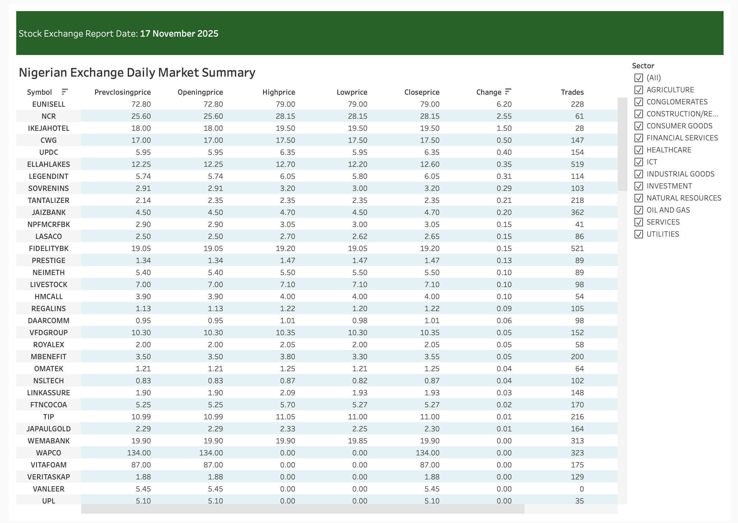
Click here to view the Nigerian stock market equity prices dashboard
The pipeline feeds multiple dashboards designed to answer specific questions:
Gap Analysis Dashboard
Purpose: Identify stocks with significant overnight price gaps
Business Value: Traders can quickly spot stocks that opened with unusual price movements, often indicating news events or institutional activity.
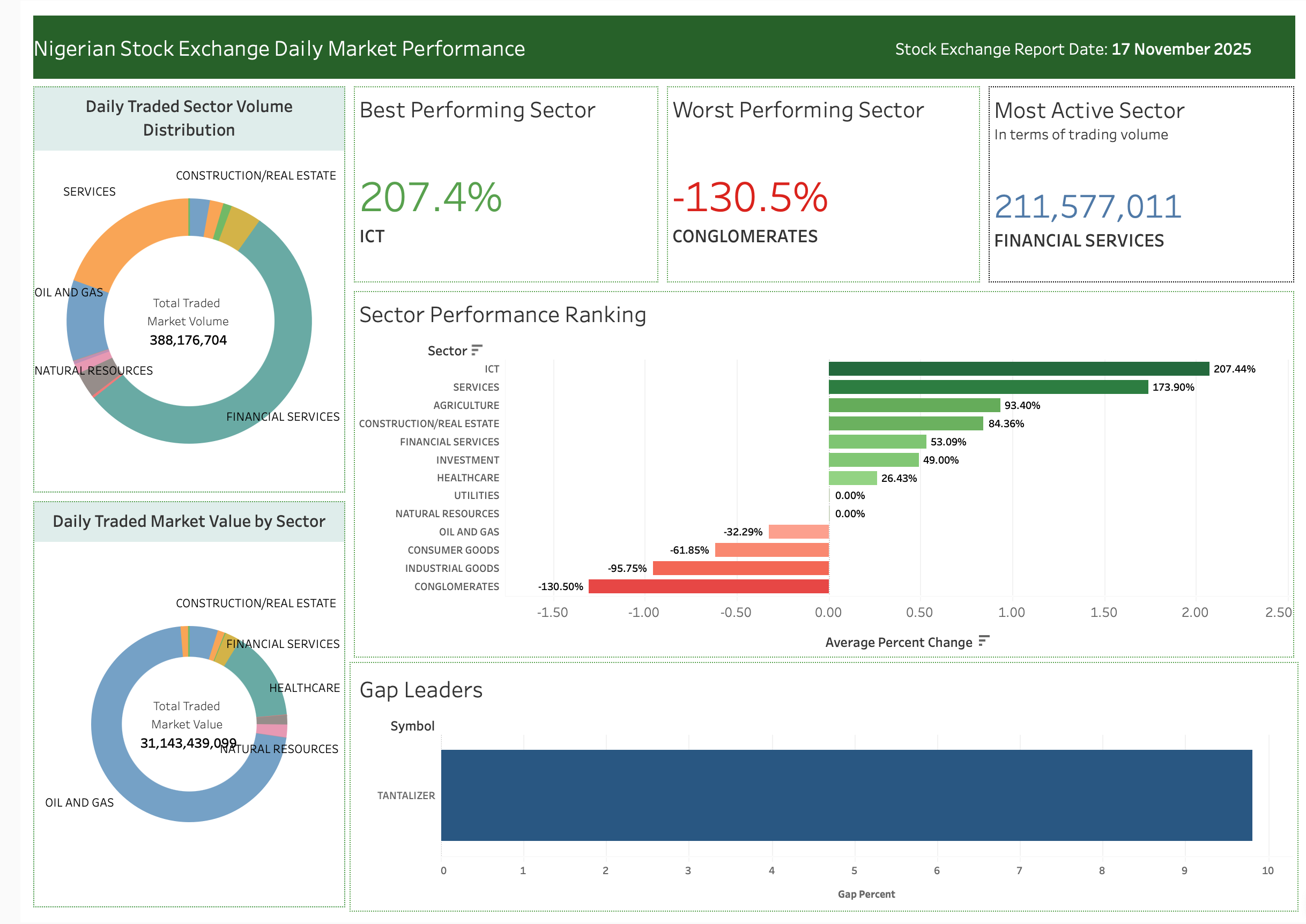
Sector Performance Dashboard
Purpose: Track relative sector strength and rotation
Business Value: Portfolio managers can identify sector rotation patterns and adjust allocations accordingly. For example, if Banking is underperforming while Industrial Goods rallies, it might signal a defensive rotation.
Top Gainers & Losers Dashboard
Purpose: Surface the day’s biggest movers
Business Value: Momentum traders can identify strong trends, while risk managers can spot unusual volatility in specific stocks.
Volume Leaders Dashboard
Purpose: Identify unusual trading activity
Business Value: High volume often precedes major price moves. Institutional accumulation or distribution typically shows up as above-average volume before the stock makes a significant move.
Market Overview Dashboard
Purpose: Comprehensive market health snapshot
Business Value: A holistic view of market sentiment. When breadth is strong (many more advancers than decliners), it indicates broad market strength rather than narrow leadership.
Technical Decisions & Trade-offs
Why Apache Airflow?
Built for data pipelines with dependency management
Excellent monitoring and alerting
Retry logic and error handling out of the box
Scales well (can distribute tasks across multiple workers)
Decision: Given the multi-step workflow with dependencies (fetch → store → refresh → export → validate), Airflow’s orchestration capabilities justify the setup overhead.
Why PostgreSQL?
Pros:
Excellent analytics performance with proper indexing
Materialized views are a first-class feature
ACID compliance ensures data integrity
Free and open-source
Cons:
Not optimized for extremely high-frequency updates (not an issue for daily batch processing)
Decision: Perfect fit for this use case. Daily batch updates, complex analytical queries, and materialized view support make PostgreSQL ideal.
Why Materialized Views Over Regular Tables?
I could have written Python/Pandas code to calculate these metrics and insert them into regular tables. Why materialized views?
Advantages:
Declarative SQL is easier to review and modify than procedural code
Automatic refresh with a single command (
REFRESH MATERIALIZED VIEW)Consistency - all views refresh from the same base table snapshot
Indexable - can add indexes for even faster queries
Less code to maintain - no Python logic for aggregations
Trade-offs:
Requires PostgreSQL (not portable to other databases without changes)
Refresh takes time (though
REFRESH MATERIALIZED VIEW CONCURRENTLYsolves this for production)
Future Enhancements
Historical Data Storage
Currently, the pipeline only keeps the latest day’s data. To enable trend analysis, I plan to:
Switch from
TRUNCATEtoINSERTwith date partitioningCreate time-series views showing week-over-week, month-over-month changes
Add moving averages and momentum indicators
Real-Time Updates
For intraday trading, daily updates aren’t enough. Enhancements could include:
Streaming data ingestion (Kafka + Flink)
Incremental materialized view refreshes
Machine Learning Integration
With historical data, we could build:
Anomaly detection (unusual volume or price moves)
Sector rotation predictions
Momentum scoring algorithms
Portfolio optimization models
Alerting & Notifications
Traders want to know immediately when:
A stock gaps up/down more than 5%
Volume exceeds 2x the average
A sector rotation occurs
I could add alerting via email or SMS.
Multi-Exchange Support
Expanding beyond NGX to include:
Other African exchanges (JSE, EGX, NSE Kenya)
Comparative analysis across markets
Currency normalization for cross-border comparisons
Conclusion
Building this NGX equities analytics pipeline taught me that great data engineering isn’t just about moving data—it’s about creating systems that deliver insights reliably and efficiently.
Key Takeaways:
Orchestration matters - Airflow turns a fragile script into a robust, monitored pipeline
Materialized views are powerful - Pre-computing queries can improve performance by orders of magnitude
Design for failure - APIs fail, networks timeout, data is messy. Handle it gracefully
Start simple, iterate - A working MVP beats a perfect plan that never ships
Visualization is the payoff - All the engineering enables one thing: better decisions
Whether you’re analyzing stock markets, e-commerce data, or IoT sensors, these patterns apply. Extract data reliably, transform it intelligently, store it efficiently, and visualize it effectively.
The complete code for this project is available on GitHub here
Let’s Connect
I’m always interested in discussing data engineering, financial analytics, and building robust pipelines. Whether you’re working on similar projects or have questions about this implementation:
If you found this useful, feel free to share it with your network. And if you’re building something similar, I’d love to hear about your approach and challenges!
All data is sourced from publicly available NGX APIs. This is for educational purposes and is not financial advice.
It's interesting how you picked this stack. Very robust pipeline. Curios about streaming options.